iNaturalist

# packages (https://statsandr.com/blog/an-efficient-way-to-install-and-load-r-packages/)

packages <- c("rinat", "tidyverse", "leaflet", "htmltools")

installed_packages <- packages %in% rownames(installed.packages())

if (any(installed_packages == FALSE)) {
  install.packages(packages[!installed_packages])
  } else {
  invisible(lapply(packages, library, character.only = TRUE)); rm(packages, installed_packages)
  }

## ── Attaching core tidyverse packages ──────────────────────── tidyverse 2.0.0 ──
## ✔ dplyr     1.1.4     ✔ readr     2.1.5
## ✔ forcats   1.0.0     ✔ stringr   1.5.1
## ✔ ggplot2   3.5.2     ✔ tibble    3.3.0
## ✔ lubridate 1.9.4     ✔ tidyr     1.3.1
## ✔ purrr     1.0.4     
## ── Conflicts ────────────────────────────────────────── tidyverse_conflicts() ──
## ✖ dplyr::filter() masks stats::filter()
## ✖ dplyr::lag()    masks stats::lag()
## ℹ Use the conflicted package (<http://conflicted.r-lib.org/>) to force all conflicts to become errors

Obter dados e metadados

lente <- rinat::get_inat_obs_project("lente-ecologica-biodiversidade-do-norte-fluminense-03ec13fb-b9dc-4175-b47e-09dce7fa5848", type = "info", raw = FALSE)

## 18970 records

# extrair registros
lente_obs <- rinat::get_inat_obs_project(lente$id, type = "observations")

## 18970 records

## Warning in rinat::get_inat_obs_project(lente$id, type = "observations"): Number of observations in project greater than current API limit.
## Returning the first 10000.

## Getting records 0-200

## Getting records up to 400

## Getting records up to 600

## Getting records up to 800

## Getting records up to 1000

## Getting records up to 1200

## Getting records up to 1400

## Getting records up to 1600

## Getting records up to 1800

## Getting records up to 2000

## Getting records up to 2200

## Getting records up to 2400

## Getting records up to 2600

## Getting records up to 2800

## Getting records up to 3000

## Getting records up to 3200

## Getting records up to 3400

## Getting records up to 3600

## Getting records up to 3800

## Getting records up to 4000

## Getting records up to 4200

## Getting records up to 4400

## Getting records up to 4600

## Getting records up to 4800

## Getting records up to 5000

## Getting records up to 5200

## Getting records up to 5400

## Getting records up to 5600

## Getting records up to 5800

## Getting records up to 6000

## Getting records up to 6200

## Getting records up to 6400

## Getting records up to 6600

## Getting records up to 6800

## Getting records up to 7000

## Getting records up to 7200

## Getting records up to 7400

## Getting records up to 7600

## Getting records up to 7800

## Getting records up to 8000

## Getting records up to 8200

## Getting records up to 8400

## Getting records up to 8600

## Getting records up to 8800

## Getting records up to 9000

## Getting records up to 9200

## Getting records up to 9400

## Getting records up to 9600

## Getting records up to 9800

## Getting records up to 10000

## Done.

## Note: mismatch between number of observations reported and returned by the API.

Mapa de registros

Mapa clássico

library(tidyverse)

lente_obs %>% 
  ggplot(aes(x = as.numeric(longitude), y = as.numeric(latitude), color = quality_grade)) +
                           # colour = scientific_name)) +
    geom_polygon(data = map_data("world"),
                 aes(x = long, y = lat, group = group),
                 fill = "grey95",
                 color = "gray40",
                 linewidth = 0.1) +
    geom_point(size = 1.2, alpha = 0.6) +
    coord_fixed(xlim = range(as.numeric(lente_obs$longitude), na.rm = TRUE),
                ylim = range(as.numeric(lente_obs$latitude), na.rm = TRUE)) +
    theme_classic() +
    theme(legend.title = element_blank()) +
    labs(x = "Longitude", y = "Latitude")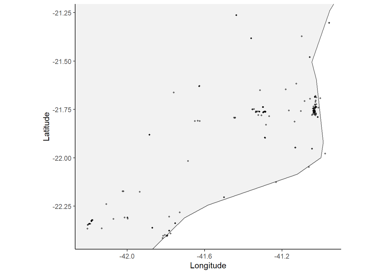

Mapa interativo

library(leaflet)

lente_obs %>% 
  leaflet() %>% 
  addTiles() %>% 
  addMarkers(~as.numeric(longitude),
             ~as.numeric(latitude),
             label = ~htmltools::htmlEscape(paste("species=", species_guess, "/", "id=", id)),
             popup = ~htmltools::htmlEscape(paste("data=", observed_on)))

Registros

Variacao temporal de registros

lente_obs %>% 
  select(observed_on, quality_grade, species_guess, user_id, quality_grade) %>% 
  mutate(ano_mes = as.POSIXct(observed_on) %>% zoo::as.yearmon()) %>% 
  group_by(ano_mes, quality_grade) %>% 
  summarise(occ = n_distinct(species_guess)) %>% 
  ggplot(aes(x = ano_mes, y = occ, fill = quality_grade)) +
    geom_bar(stat = "identity") +
    theme_classic() +
    labs(x = "", y = "registros (n)")

## `summarise()` has grouped output by 'ano_mes'. You can override using the
## `.groups` argument.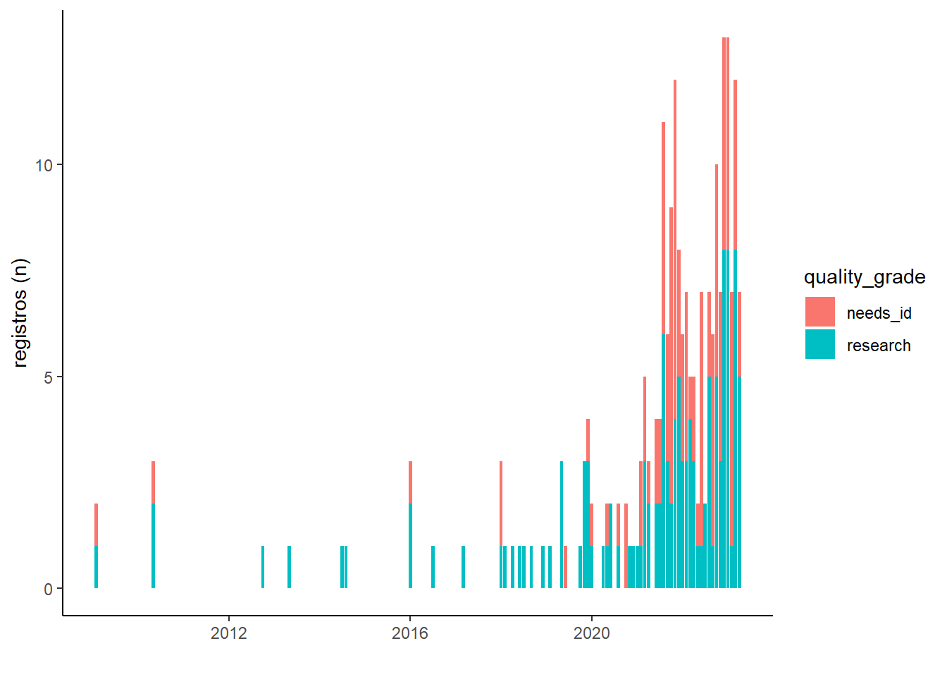

Registros por usuario

# ordenar
ordem <- lente_obs %>% 
  select(observed_on, quality_grade, species_guess, user_id, quality_grade) %>% 
  mutate(ano_mes = as.POSIXct(observed_on) %>% zoo::as.yearmon()) %>% 
  group_by(user_id) %>% 
  summarise(occ = n_distinct(species_guess)) %>%
  arrange(-occ) %>% pull(user_id)

# grafico
lente_obs %>% 
  select(observed_on, quality_grade, species_guess, user_id, quality_grade) %>% 
  mutate(ano_mes = as.POSIXct(observed_on) %>% zoo::as.yearmon()) %>% 
  group_by(user_id, quality_grade) %>% 
  summarise(occ = n_distinct(species_guess)) %>%
  arrange(-occ) %>% 
  ggplot(aes(y = occ, x = factor(user_id, levels = ordem), fill = quality_grade)) +
    geom_bar(stat = "identity") +
    theme_classic() +
    theme(axis.text.x = element_text(angle=90, hjust=1, vjust=0.5),
          legend.title = element_blank()) +
    labs(x = "", y = "registros (n)")

## `summarise()` has grouped output by 'user_id'. You can override using the
## `.groups` argument.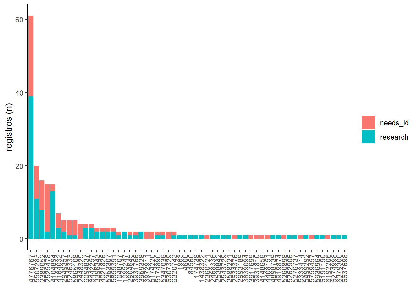

Colabore, compartilhe, e cite as fontes!